High-performance derivative calculation techniques for scientific computing

post under construction 🚧

Automatic differentiation is a fundamental component of modern deep learning. Numerous powerful implementations exist in Python, but here we focus on the methods implemented in JAX - a stable and robust library develop by Google.

All code examples are available in Colab.

Finite differences is not autodiff

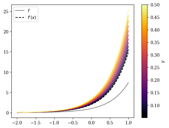
Given the function \(f(x)=\exp(2x)\), it’s exact derivative is \(f^{\prime}(x)=2\exp(2x)\). From a computational perspective, we can approximate the derivative using the finite difference ratio given by

\[Df(x):=\frac{f(x+\gamma)-f(x)}{\gamma}\]

where \(\gamma\) is a small positive number.

In the following example, we construct the functions \(f(x)\), \(f^{\prime}(x)\), and \(Df(x)\). After implementing these functions, we analyze the behavior of the exact derivative compared to the approximate derivative obtained using finite differences. The Figure below shows that varying \(\gamma\) can significantly affect the final results.

As expected, the larger the value of \(\gamma\), the further the approximation diverges from the exact derivative.

Symbolic calculus is not autodiff

Another strategy for computing derivatives is symbolic calculus. However, this approach is not well-suited for high-performance computing, and a key drawback is its inability to differentiate through control flow structures, such as conditional statements or loops.

In the following example, we’re using symbolic calculus with Python’s sympy library to compute the 6th-order derivative of a function \(f(x) = (a \cdot x + b)^m\).

m, a, b, x = symbols('m a b x')
f_x = (a*x + b)**m
f_x.diff((x, 6)) # 6-th order derivative

\[a^{6}m(ax + b)^{m}(m{5} - 15m^{4} + 85m^{3} - 225m^{2} + 274m - 120)/(ax + b)^{6}\]

symbols('m a b x') creates symbolic variables \(m\), \(a\), \(b\), and \(x\). These are placeholders that can represent constants or variables for calculus operations;
f_x = (a*x + b)**m is defined as a symbolic expression. Here, \(a\) and \(b\) are parameters, \(m\) is an exponent, and \(x\) is the variable of differentiation;
f_x.diff((x, 6)) computes the 6th derivative of \(f(x)\) with respect to \(x\). Higher-order derivatives like this require differentiating the function 6 times;
The result will be a symbolic expression representing the 6th derivative. Depending on the values of \(a\), \(b\), and \(m\), this expression may grow quite large. SymPy will leave the result in symbolic form unless you further simplify or evaluate it;

Symbolic calculus with sympy allows for exact, algebraic manipulation of functions, which is useful when precision is needed or when working with general forms of derivatives that can’t be easily solved numerically.

The autodiff approach

Automatic differentiation (autodiff) generates functions that compute derivatives at specific numerical inputs provided by the calling code, rather than producing a single symbolic expression for the entire derivative. In this process, the derivative is constructed incrementally by decomposing the original computation into simpler components using the chain rule

\[\frac{d}{dx} f(g(x)) = f'(g(x)) \cdot g'(x).\]

The chain rule is repeatedly applied to propagate derivatives through all intermediate operations, down to elementary functions such as addition, subtraction, multiplication, division, exponentiation, and trigonometric functions (e.g., \(\sin(x)\), \(\cos(x)\)). These elementary operations are analytically differentiable, allowing the program to compute their derivatives exactly.

Since autodiff operates at a graph level, it constructs a computational graph of the function, with nodes representing intermediate values and edges representing dependencies. By following the graph, it efficiently applies the chain rule in either forward mode or reverse mode, depending on the desired performance and dimensionality of the problem.

Some math and code on autodiff

Following, we use the insights provided by Autodiff with JAX notebook.

Consider the function \(f : \mathbb{R}^n \to \mathbb{R}^m\). The Jacobian of \(f\) evaluated at the point \(x \in \mathbb{R}^n\) is the matrix

\[\partial{f}(x) = \begin{bmatrix} \frac{\partial f_1}{\partial x_1}(x) & \frac{\partial f_1}{\partial x_2}(x) & \cdots & \frac{\partial f_1}{\partial x_n}(x) \\ \frac{\partial f_2}{\partial x_1}(x) & \frac{\partial f_2}{\partial x_2}(x) & \cdots & \frac{\partial f_2}{\partial x_n}(x) \\ \vdots & \vdots & \ddots & \vdots \\ \frac{\partial f_m}{\partial x_1}(x) & \frac{\partial f_m}{\partial x_2}(x) & \cdots & \frac{\partial f_m}{\partial x_n}(x) \end{bmatrix} = \left[\frac{\partial f_i}{\partial x_j}(x)\right]_{i=1,j=1}^{m,n} \in \mathbb{R}^{m \times n}.\]

As for any matrix, the Jacobian \(\partial{f}(x) : \mathbb{R}^n \to \mathbb{R}^m\) is a linear map \(v \mapsto \partial{f}(x)v\) defined by the usual matrix-vector multiplication rules.

Autodiff uses pre-defined derivatives and the chain rule to compute derivatives of more complex functions. In particular, autodiff can be used to compute the Jacobian-Vector Product (JVP)

\[\begin{aligned} \partial{f}(x) : \mathbb{R}^n &\to \mathbb{R}^m \\ v &\mapsto \partial{f}(x)v \end{aligned}\]

and the Vector-Jacobian Product (VJP)

\[\begin{aligned} \partial{f}(x)^\top : \mathbb{R}^m &\to \mathbb{R}^n \\ w &\mapsto \partial{f}(x)^\top w \end{aligned}\]

The maps \(v \mapsto \partial{f}(x)v\) and \(w \mapsto \partial{f}(x)^\top w\) are also known as the pushforward and pullback, respectively, of \(f\) at \(x\). The vectors \(v\) and \(w\) are termed seeds in autodiff literature.

Given the function composition

\[h(x) = (f_N \circ f_{N-1} \circ \cdots \circ f_1)(x) = f_N(f_{N-1}(\cdots f_1(x)\cdots)),\]

where each \(f_k : \mathbb{R}^{d_k} \to \mathbb{R}^{d_{k+1}}\) is some differentiable map.

We can write this recursively as

\[y_0 = x \in \mathbb{R}^n,\quad y_{k+1} = f_k(y_k) \in \mathbb{R}^{d_{k+1}},\quad y_N = h(x) \in \mathbb{R}^{d_N}.\]

By the chain rule, we have

\[\partial{h}(x) = \partial{f_N}(y_{N-1})\partial{f_{N-1}}(y_{N-2}) \cdots \partial{f_1}(y_0).\]

This sequence of matrix multiplications that can get quickly get expensive for complicated functions.

It is more efficient and usually sufficient in practice to compute JVPs via the recursion

\[\begin{aligned} \partial{h}(x)v_0 &= \partial{f_N}(y_{N-1})\partial{f_{N-1}}(y_{N-2}) \cdots \partial{f_1}(y_0) v_0 \\ &= v_N \\ v_k &= \partial{f_k}(y_{k-1})v_{k-1} \end{aligned},\]

and VJPs via the recursion

\[\begin{aligned} \partial{h}(x)^\top w_0 &= \partial{f_1}(y_0)^\top \cdots \partial{f_{N-1}}(y_{N-2})^\top \partial{f_N}(y_{N-1})^\top w_0 \\ &= w_N \\ w_k &= \partial{f_{N-k+1}}(y_{N-k})^\top w_{k-1} \end{aligned}.\]

VJPs require more memory than JVPs, since \(\{y_k\}_{k=1}^{N-1}\) must be computed and stored first (i.e., the forward pass) before recursing (i.e., the backward pass).

Simple example

Given the function

\[f(x)=\sin(x)-2\cos(3x)\exp(-x^{2})\]

it’s exact derivative is

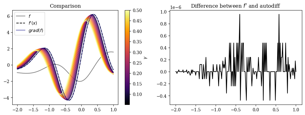
\[f^{\prime}(x)=\cos(x) + 6\sin(3x)\exp(-x^{2}) + 4x\cos(3x)\exp(-x^{2})\]

We can visualize the \(f\), \(f^{\prime}(x)\), \(Df_{0.1}\), and the \(grad(f)\) as

Differentiating through control flow

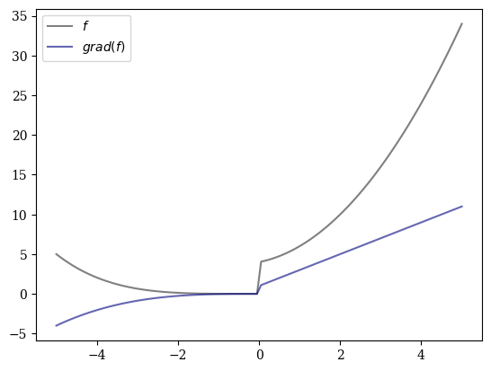
Given a piecewise function \(f(x)\) with two nested sub-functions. If \(x < 0\), the function \(f_1(x)\) is applied, iteratively modifying \(x\) by scaling it in a loop. Otherwise, the function \(f_2(x)\) is used, which computes the sum of \(x^i + i\) for \(i\) ranging from 0 to 2. The gradient of \(f\), \(f^{\prime}(x)\), is computed using jax.grad. Both function \(f(x)\) and its gradient over a grid of 100 points from -5 to 5, with the function curve shown in gray and its gradient in navy blue.